Sinewave deconvolution

Many time-dependent phenomena show a periodic behaviour. This can arise from one or more oscillatory component, often summed up with a linear trend. Example of this are the sunspot number, with a periodicity of about 11 years. Other examples comprise the neutron flux deriving from the cosmic rays impinging over the atmosphere, the solar radio flux at 10.7 GHz and many others.

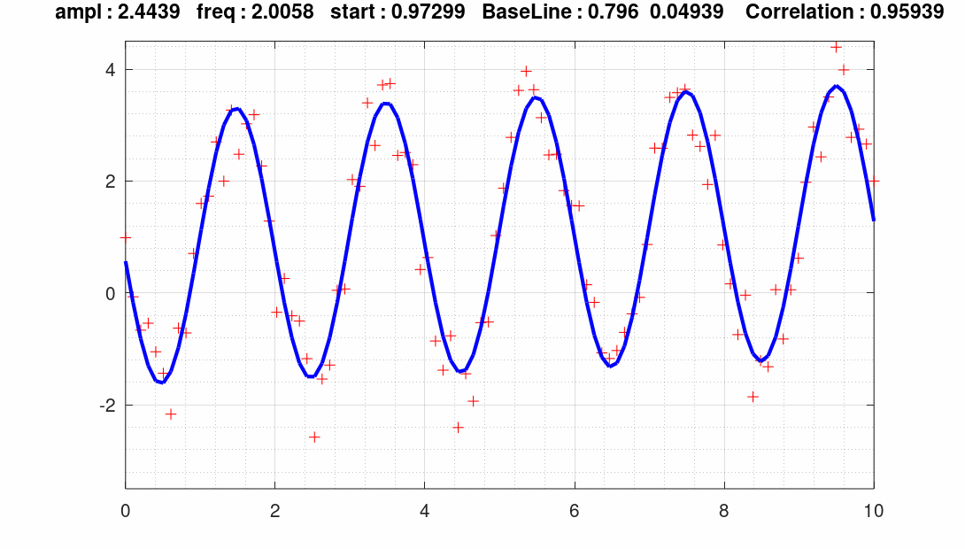
The example below shows how to deconvolve noisy data with a periodic trend superimposed to a linear slope.

SCRIPT : (www.octave.org)

clc;clear all;

global x10 y10

function delta = effe(p); % MINIMIZING FUNCTION

global x10 y10

y = sinewave(x10,p);

delta = sumsq(y - y10);

endfunction

function y = sinewave(x10,p); % INTERPOLATING FUNCTION = sinewave + linear trend

y = p(1)*sin(2*pi/p(2)*(x10 - p(3))) + p(4) + p(5)*x10;

endfunction

% Some random data are generated and plotted

x10 = linspace (0,10,100)';y10 = zeros(100,1);

p0(1) = 2.5; % amplitude

p0(2) = 2; % period

p0(3) = 1; % start sin(x)

p0(4) = 0.05 % baseline (constant value)

p0(5) = 0.08 % baseline (coeff 1° degree)

y10 = sinewave(x10,p0);

y10 = y10 + 2*rand(100,1)-0.5;

figure (1,'position',[200 100 700 400]);

plot(x10,y10,'r','marker','+','linestyle','none'); % points

axis([0 10 -3.5 4.5]);grid on;grid minor on;hold on;

% fMinSearch on the sum of squares of delta

fer = @(p) effe(p);

[p1,fer1] = fminsearch(fer,p0);

% final plot

y11 = sinewave(x10,p1);

plot(x10,y11,'b','linewidth',2);

title(["ampl : ",num2str(p1(1))," freq : ",num2str(p1(2))," start : ",num2str(p1(3))," BaseLine : ",num2str(p1(4))...

," ",num2str(p1(5))," Correlation : ",num2str(corr(y10,y11))]);