Sigmoid curve

A sigmoid function is a mathematical function having a characteristic "S"-shaped curve. A common example of a sigmoid function is the logistic function defined by the formula:

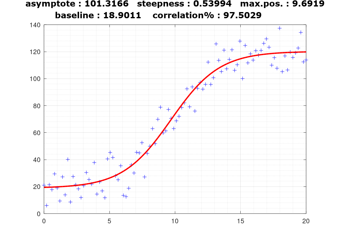
The more general form here employed, uses four parameters :

where ‘a’ = asymptot, ‘b’ = skewness, ‘c’ = abscissa of mid point and ‘d’ = background baseline.

SCRIPT : (www.octave.org)

clc;clear all;

global x10 y10

function delta = sigmoid(p);

global x10 y10

y = p(1)./(1 + exp(-p(2)*(x10 - p(3)))) + p(4);

delta = sumsq(y - y10);

endfunction

p0(1) = 95 %100 asymptot

p0(2) = 0.56 %0.5 skewness

p0(3) = 10 %0.1 a/2 abscissa

p0(4) = 17 %20; Baseline (constant value)

% generation of noisy data

x10 = linspace (0,20,100)';

y10 = 100./(1 + exp(-0.5*(x10 - 10))) + 20 + 10*randn(100,1);

[p1,fer1] = fminsearch("sigmoid",p0);

figure (1,'position',[200 100 700 500]);

plot(x10,y10,'b+');

axis([0,20,0,140]);grid on;grid minor on;hold on;

y11 = p1(1)./(1 + exp(-p1(2)*(x10 - p1(3)))) + p1(4);

plot(x10,y11,'r','linewidth',2);

title(["asymptote : ",num2str(p1(1))," steepness : ",num2str(p1(2))," max.pos. : ",num2str(p1(3));" baseline : ",num2str(p1(4))," correlation% : ",num2str(100*corr(y10,y11))],'fontsize',13,'fontname','verdana');

In 1976, after several decades of relative stability, the Earth’s surface abruptly began to warm. According to AGW proponents the warming since then has been effectively straight-line, i.e. more or less what we would expect from increasing atmospheric CO2 concentrations. There is, however, another explanation that fits observations at least as well if not better – that the warming actually proceeded in a series of upward steps, with temperatures increasing only during major El Niño/La Niña events. And the cause? Releases of surplus heat from the ocean during these Niño/Niña events. This evidence has been named “Staircase Hypothesis”.