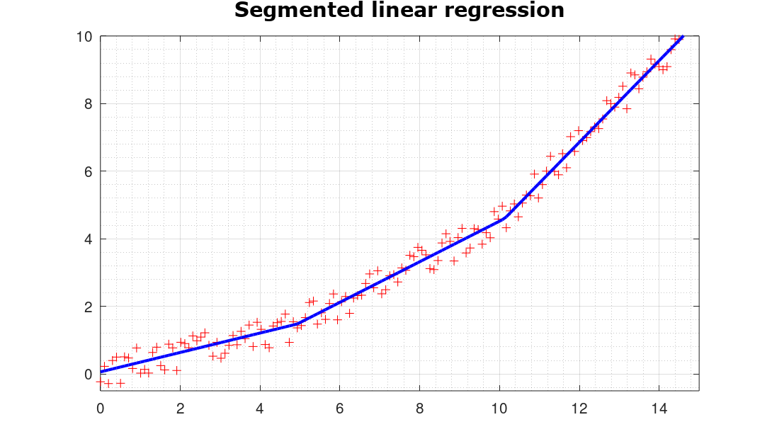
Segmented regression

The most common form of regression analysis is the linear regression, which can be segmented as well. One finds the line that most closely fits the data according to a specific mathematical criterion. For example, the method of ordinary least squares computes the unique line that minimizes the sum of squared differences between the true data and that line itself.

Quite often linear regression is applied to the whole available data set or to a part of it, aiming to evidence some particular trend in a given time range. The choice of the time range used is often quite arbitrary.

Given a set of n equally time-spaced observations, it is known that the slope of the regression line b is given by where indicate mean values .

SCRIPT : (www.octave.org)

clear all;clc;format short;format compact;

global x10 y10 y11

function delta = effe(p); % MINIMIZING FUNCTION

global x10 y10 y11

pp = splinefit(x10,y10,[x10(1) p(1) p(2) x10(end)],"order",1);

y11 = ppval(pp,x10);

delta = sumsq(y11 - y10);

endfunction

% Some random data are generated and plotted

x10 = linspace (0,15,150)';y10 = zeros(150,1);

y10(1:50) = 0.3*x10(1:50);

y10(51:100) = 0.6*x10(51:100) - 1.5;

y10(101:150) = 1.2*x10(101:150) - 7.5;

y10 = y10 + rand(150,1)-0.5;

figure (1,'position',[200 100 700 400]);

plot(x10,y10,'r','marker','+','linestyle','none'); % points

axis([0 15 -0.5 10]);grid on;grid minor on;hold on;

% Start Guess is defined (2 parameters)

p0(1) = 6;

p0(2) = 11;

% fMinSearch on the sum of squares of delta

[p1,fer1] = fminsearch('effe',p0);

pp = splinefit(x10,y10,[x10(1) p1(1) p1(2) x10(end)],"order",1);

qq = struct2cell(pp);

for k=1:3;m(k) = qq{3}(k,1);endfor

% Segmented regression is plotted

plot(x10,y11,'b','linewidth',2);

title('Segmented linear regression','fontname','verdana','fontsize',14);

printf ("from x = %.3f to x = %.3f slope is = %.3f \n", [x10(1) p1(1) m(1)]);

printf ("from x = %.3f to x = %.3f slope is = %.3f \n", [p1(1) p1(2) m(2)]);

printf ("from x = %.3f to x = %.3f slope is = %.3f \n", [p1(2) x10(end) m(3)]);

disp(['correlation : ',num2str(corr(y10,y11))]);

------------------------------------------------------

OUTPUT :

from x = 0.000 to x = 4.932 slope is = 0.287

from x = 4.932 to x = 10.128 slope is = 0.601

from x = 10.128 to x = 15.000 slope is = 1.207

correlation : 0.99565