Periodicity analysis

Many climatological data have a periodic (evident of hidden) oscillation. For example if temperatures are referred to a part of the globe these are subject to yearly periodic variations. Under other circumstances solar cycles (like the 11-years Schwabe cycle) are responsible for periodic variations.

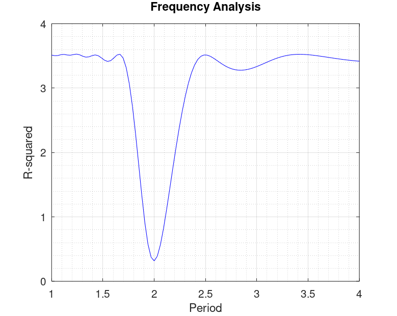
In order to look for periodic signals, there are several mathematical tools. A periodogram is one of them. A periodogram calculates the significance of different frequencies in time-series data to identify any intrinsic periodic signals. In this respect it is similar to the Fourier Transform, but is optimized for unevenly time-sampled data, and for different shapes in periodic signals. Many different frequencies and candidate periodic signals are evaluated, and the statistical significance of each frequency is computed based upon a series of algebraic operations that depend on the particular algorithm used and periodic signal shape assumed. As a result, any physical waveform can be decomposed into a number of discrete frequencies, or a spectrum of frequencies over a certain range.

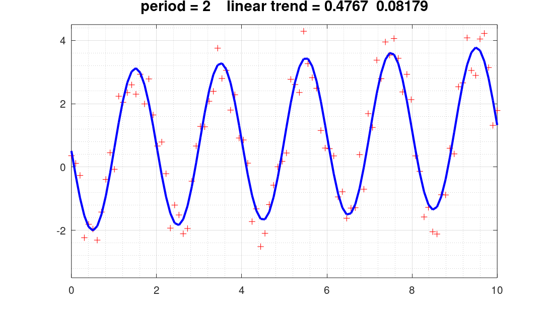
SCRIPT : (www.octave.org)

clc;clear all;

global x10 y10 xd Ud;

function sd = best(pr) % ------ minimizer according to least square summation

global x10 y10 xd Ud;

Ud(:,3) = sin(2*pi/pr*x10); % sin

Ud(:,4) = cos(2*pi/pr*x10); % cos

[xd,sd,rd] = ols(y10,Ud); % ols = Ordinary Least Square refinement

endfunction % ------ end of minimizer

function y = sinewave(x10,p); % INTERPOLATING FUNCTION = sinewave + linear trend

y = p(1)*sin(2*pi/p(2)*(x10 - p(3))) + p(4) + p(5)*x10;

endfunction

% Some noisy sinewave data are generated

x10 = linspace (0,10,100)';

p0(1) = 2.5; % amplitude

p0(2) = 2; % period

p0(3) = 1; % start sin(x)

p0(4) = 0.05; % baseline (constant value)

p0(5) = 0.08; % baseline (coeff 1° degree)

y10 = sinewave(x10,p0);

y10 = y10 + 2*rand(100,1)-0.5;

% Ud is initialized

Ud = zeros(100,4);

Ud(:,1) = 1; % baseline, constant value

Ud(:,2) = x10; % slope (linear trend)

% Search for frequency component (search between period Limit1 and Limit2)

k = 0;Limit1 = 1;Limit2 = 4;

for m = linspace(Limit1,Limit2,100); % frequency is spanned

++k;xL(k,1) = m;pL(k,1) = best(m);

endfor

[n,in] = min(pL);Fbest = xL(in);

figure(1,'position',[100 100 500 400]);axis([Limit1,Limit2]);

plot (xL,pL,'b');grid on;grid minor on;hold on;

xlabel ('Period');ylabel ('R-squared');title ('Frequency Analysis');

x2 = best(Fbest);

figure(2,'position',[200 100 700 400]);

plot(x10,y10,'r','marker','+','linestyle','none'); % points

axis([0 10 -3.5 4.5]);grid on;grid minor on;hold on;

yN = xd(1) + xd(2)*x10 + xd(3)*sin(2*pi/Fbest*x10) + xd(4)*cos(2*pi/Fbest*x10);

plot(x10,yN,'b','linewidth',2)

title(['period = ',num2str(Fbest,3),' linear trend = ',num2str(xd(1),4),' ',num2str(xd(2),4)],'fontsize',14);