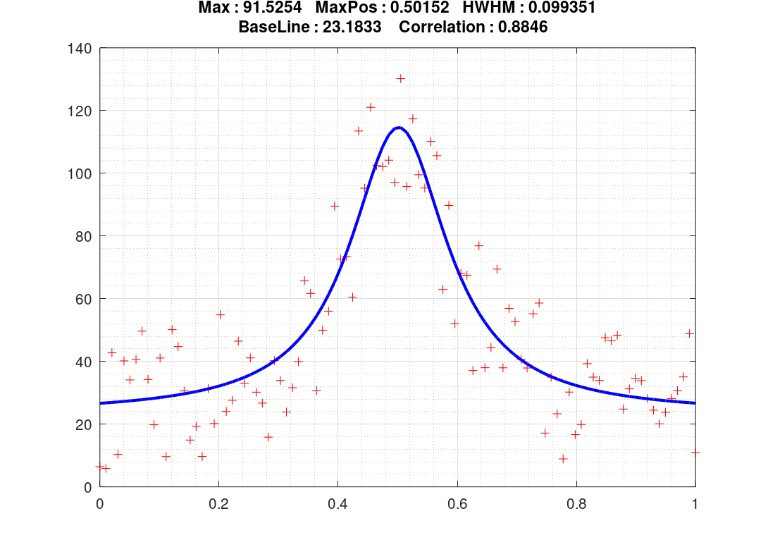
Lorentz (Cauchy) distribution

The Cauchy distribution, named after Augustin Cauchy, is a continuous probability distribution. It is also known, especially among physicists, as the Lorentz distribution (after Hendrik Lorentz), Cauchy–Lorentz distribution, Lorentz(ian) function, or Breit–Wigner distribution. It has the form:

where ‘a’ is the maximum value, ‘b’ is the maximum position (abscissa), ‘c’ is the Half Width at Half Maximum (HWHM) and ‘d’ the background constant value.

The following script is an example of lorentz interpolation. It generates some noisy data and interpolates them with a lorentz curve. It is used in this web-site here for various climatological dataset interpolation.

SCRIPT : (www.octave.org)

clc;clear all;

global x10 y10

function delta = Cauchy(p);

global x10 y10

y = p(1)./(1 + ((x10 - p(2))./p(3)).^2) + p(4);

delta = sumsq(y - y10);

endfunction

p0(1) = 95; %100 Maximum intensity

p0(2) = 0.56; %0.5 Maximum position (x axis)

p0(3) = 0.15; %0.1 HWHM

p0(4) = 17; %20; Baseline (constant value)

x10 = linspace (0,1,100)';

y10 = 100./(1 + ((x10 - 0.5)./.1).^2) + 20 + 50*(rand(100,1)-0.5);

[p1,fer1] = fminsearch("Cauchy",p0);

figure (1,'position',[200 100 700 500]);

plot(x10,y10,'r','marker','+','linestyle','none');

axis([0,1,0,140]);grid on;grid minor on;hold on;

y11 = p1(1)./(1 + ((x10 - p1(2))./p1(3)).^2) + p1(4);

plot(x10,y11,'b','linewidth',2);

title(["Max : ",num2str(p1(1))," MaxPos : ",num2str(p1(2))," HWHM : ",num2str(p1(3));" BaseLine : ",num2str(p1(4))...

," Correlation : ",num2str(corr(y10,y11)) ]);

disp(['correlation = ',num2str(corr(y10,y11))]);

disp(['spearman = ',num2str(spearman(y10,y11))]);

disp(['kendall = ',num2str(kendall(y10,y11))]);